When it comes to business, Microsoft’s Excel is a powerful tool that can be used to crunch the numbers and analyze the data in ways that can save time and money. With Excel there seems to be no middle ground in the debate of whether to love it or despise it.
That said, though, with a proper understanding of this incredible tool, we are sure that you will be able to find it not only useful but be able to improve on your experience with it and thus end up loving it as so many others do.
Excel isn’t nearly as complicated as many people make it out to be (and perhaps even how you see it yourself), as long as you have the basics and understand them. Once you do, you should be able to navigate through the pages of data and be able to explore a few more tips and tricks you didn’t know you needed until now.
1. Using the Sum Function
Of all the functions in Excel, this is probably the one used the most, as it is the most basic but also the most needed. The sum function, as its name would give you to believe, is used to calculate the total sum of the selected cell values.
For instance, if you would like to know what the total amount was that you spent over the weekend during that spur-of-the-moment getaway, all you would need to do would be to left-click on the cell where the answer needs to be and simply type in the formula =SUM (B1:B14) and hit the Enter key.
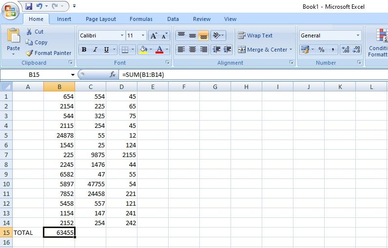
You can use the Sum function for any column with numerical value and if you only want to add up certain of the cells in that column you can do so by typing in =Sum (B1+B4+B7) and then hitting the Enter key.
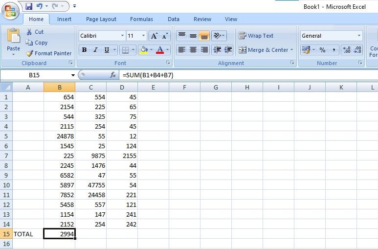
Naturally, the cell numbers you want to add up will be the ones you type in the area between brackets, whether it is C5, F6 or G3 etc.
2. Sorting the Data
Spreadsheets are a fantastic way of sorting through lots and lots of data as well as enabling you to keep your data neat and in order. For example, if you would like to know how much an employee spent whilst on a job during that month, you could simply highlight the entire sheet by selecting all the cells, and then you would left-click on the Data tab at the top of the page and then select Filter.
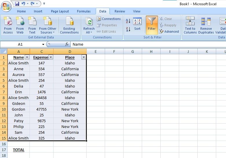
To sort according to employee, you can now left-click on the little drop down menu arrow next to the employee name and select only the employee whose data you would like to see. This will then show you only that employee’s records, allowing you to work out the total by using the Sum function as discussed in the first point.
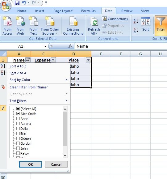
You can use this sorting function to sort your sheet according to your preference. You can also take off the sorting function by selecting the entire sheet and then going to Data and simply de-selecting the Filter function.
3. Sizing Things Up
Changing the size of columns and rows is something you will also find yourself doing very often during your use of Excel. You can make changes to the size of your columns or rows by letting your mouse hover on the border of the column/row you wish to resize and then left-click and drag the pointer to make the column/row bigger or smaller.
If you have typed data into the cells and you can’t view it all, simply double-click on the border of the column/row and it will automatically resize to fit the contents.
4. How to Remove Unnecessary Cells or Columns
Perhaps you have had to make a few changes to one or two departments in the company and you find that you now have some empty columns or cells that you no longer need. Should you need to remove a column, all you need to do is to highlight/select the column in question, right-click on it and then select Delete.
On the other hand, you could also highlight the unwanted column and then in the top pane, select the Home tab and then go left-click on the Delete button which is located on the right-hand side of the screen.
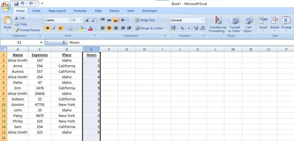
You can then select Delete Sheet Columns or you can select the cells which you would like to delete and select Delete Cells. You will then need to select Shift Cells Left and then click on Ok.
Should you wish to add an extra column or cell, simply left-click on the place where you would like the extra column or cell to appear, then select the Insert tab at the top of the page and select Insert Sheet Column or Insert Cells.
5. Freezing the Panes
If you have a big spreadsheet with lots of information on it and you want to be able to view certain cells that are further along without having to constantly scroll back and forth, there is a nifty little trick you can perform which will sort the problem for you. It’s called Freeze Pane.
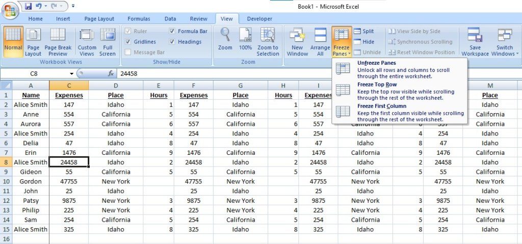
For instance, if you would like to keep a particular cell or column in sight at all times, select the row or column where the data you want to keep in sight begins. Then left-click on the View tab at the top of the screen. Then you will select the Freeze Panes menu and from the drop down menu which appears you will choose the option that suits your needs.
6. Using Charts
Let’s be honest, using a well placed pie chart gives you the ability to visually present all the data you have accumulated in a very pleasing way. And Excel has just the right amount of charts to choose from. Simply select the columns you want to add into your chart, then left-click on the Insert tab and then select See All Charts.
There are a plethora of charts to choose from and once you have decided on the kind of chart you would like, select it and then click on OK. Should you wish to move the chart to a different sheet in your Excel book, simply left-click on the chart and then in the top right-hand side of the page you can select Move Chart and then choose where you would like to move it to.
7. Getting Rid of Duplicates
No matter how careful you are, there are bound to be times when duplicates will slip in unseen. To make sure you keep on top of it and get rid of those unwanted duplicates, simply highlight your entire sheet, select the Data tab at the top of the page, then select Remove Duplicates and choose where you want to remove the duplicates from.
You will need to make sure that you make a big enough selection to ensure that you weed out the real duplicates — sometimes column A may have some identical first names or names of places but the information in the succeeding rows are different. The aim is to ensure that you weed out true duplicates, so be sure to use enough qualifiers.
8. Using Special Formatting In Cells
If you need to change the formatting in some of the cells to monetary value, for instance, you can do so with just a few simple clicks of the mouse. Select the cell you need to format, and then select the Numbers tab.
Select the Currency option and then select the currency you need to use from the drop down menu. You will see that there are more options if there is some other formatting you need to apply to the cells. You can also apply changes to more than one cell at a time if you highlight all the cells you wish to apply the change to and then make the changes, instead of making these changes to one cell at a time.
9. How to Show the Formulas
You’ve added formulas into your spreadsheet but you need to see exactly what you have done and which formulas you have inserted in which cells. Nothing could be simpler.

Just navigate to the Formulas tab at the top of the page and then left-click on Show Formulas. Now every formula you have added into your sheet will be visible to you.
10. Protecting Cells
One thing you will probably want to do is make sure that if you have to share your workbook with others that no unwanted changes can be made. Navigate to the Review (or Format) tab at the top of the page and then select Protect Sheet.
You can decide whether or not you want to allow anyone to make any modifications to your sheet, otherwise you can just enable protection on all the cells so that no changes can be made.
Choose a password and then re-enter the password to confirm. Once you have done this you will be able to rest assured that nobody will be able to make any changes to your spreadsheet and all information will be safe and secure.
You can also select Protect Workbook should you wish to protect the entire workbook and not just some of the information. Remember to write the password somewhere safe, just in case.
The Final Word … (Undo command)
We do have one last thing we would like to add before concluding, and that is that before you make any changes to your spreadsheets, always remember to make a backup copy of them first.
Let’s be honest, you never know when you may want the information and it’s so much better to be safe rather than sorry. Added to that, if you make a mistake or delete something which you find you needed later on, you will be able to go back and get the information from an older, saved copy.
You can also use the very useful CTRL Z to undo something you have just done if you made a mistake, but did you know you can press CTRL SHIFT + together and get a shortcut to inserting cells or columns.
There are just so many possibilities in Excel, so many things one can do! To really get the most out of your Excel experience, though, it’s definitely worth it to get these few functions under your belt and remember them as they will certainly help you to be able to maximize your time on Excel.
As always, if you’re needing any kind of additional help either understanding or implementing any of the Microsoft Excel functions presented in this blog post, consider reaching out to HelpCloud technicians for remote support.
